While I was glancing at hypothesis tests, I saw paired and two-sample t-test but couldn't understand the difference. For the explanation of these two tests, I saw the following sentence " Two-sample t-test is used when the data of two samples are statistically independent, while the paired t-test is used when data is in the form of matched pairs." How are these two tests are different? Because based on this explanation, I thought, we could think of the matched-pairs population as two independent populations. Can anyone explain? I only have a statistics experience of 1 year so please consider that I may have a hard time understanding profound explanations.
In a two-sample test, you have two independent samples. Of course, by independence, we expect the two sets of measurements will not be correlated. Sample sizes for the two samples need not be equal. (But it often makes sense for them to be approximately equal.)
In a paired test you have one sample of pairs. Typically, there will be $n$ paired observations $(x_i, x_2).$ These may be two measurements on each individual subject. (For example, Before and After 'treatment' scores on a questionnaire, exam, or lab test.) Alternatively, the pairs may be pairs of subjects. (For example, married couples, twins, or subjects matched according to some criterion. They might also be two devices manufactured at the same time and place.) It is expected that the two measurements on pairs will be correlated. In analysis, one may look at a sample of differences $d_i = x_1-x_2.$
Paired. Suppose you have a study in which subjects have diverse skills at a particular task. It is claimed that a training course will increase skills by a small, but important amount. You test 20 subjects before (test score x1 ) and after ( x2 ) the training.
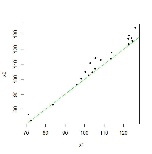
summary(x1) Min. 1st Qu. Median Mean 3rd Qu. Max. 71.16 99.70 105.31 105.91 122.32 125.95 length(x1); sd(x1) [1] 20 # sample size [1] 16.33155 # sample standard deviation summary(x2) Min. 1st Qu. Median Mean 3rd Qu. Max. 72.63 102.04 111.76 109.16 123.90 134.25 length(x2); sd(x2) [1] 20 [1] 17.30927 The average score increases from 105.91 Before training to 109.16 After. Before and after scores are highly correlated.
cor(x1,x2) [1] 0.9859222 A scatterplot shows the strong linear correlation. Also, most of the $(X_,X_)$ points lie above the 45-degree line, indicating modest, but mostly positive results from the training course.

A paired t test in R, tests $H_0: \mu_B = \mu_A$ against the one-sided alternative $H_0: \mu_B < \mu_A.$ The P-value (near $0)$ shows that the observed improvement is highly significant.
t.test(x1, x2, pair=T, alt="less") Paired t-test data: x1 and x2 t = -4.8675, df = 19, p-value = 5.347e-05 alternative hypothesis: true difference in means is less than 0 95 percent confidence interval: -Inf -2.095359 sample estimates: mean of the differences -3.249817 The pairing has allowed us to detect a small improvement 'above the noise' of great subject variability.
Two-samples. By contrast, suppose we gave the training to a group of 20 randomly chosen subjects obtaining test scores t . For comparison we taka a group of 20 subjects from the same population who did not take the training course. Also, suppose the true mean score of subjects with the training is 4 points above the true mean score of subjects who did not take the training.
Then we would have a one-sided, two-sample t test. And, we would have only about a 20% chance of detecting the difference, on account of the diversity of skills in the population.
set.seed(516) pv = replicate(10^4, t.test(rnorm(20, 100, 15), rnorm(20, 104, 15), alt="less")$p.val) mean(pv < 0.05) [1] 0.2043 Note: In the simulation above 10,000 two-sample tests are performed on samples of size $n_1=n_2=20$ from populations $\mathsf(100, 15)$ and $\mathsf(104, 15),$ respectively. The data summary and the Welch 2-sample t test are shown for the first one of these 10,000 simulated experiments.
set.seed(516) u = rnorm(20, 100, 15); u = rnorm(20, 104, 15) summary(u); length(u); sd(u) Min. 1st Qu. Median Mean 3rd Qu. Max. 85.29 101.01 111.27 110.69 120.35 134.40 [1] 20 [1] 13.30721 t = rnorm(20, 100, 15); t = rnorm(20, 104, 15) summary(t); length(t); sd(t) Min. 1st Qu. Median Mean 3rd Qu. Max. 75.96 93.48 109.83 106.62 115.34 135.87 [1] 20 [1] 15.66145 boxplot(u, t, horizontal=TRUE, col="skyblue2", names=TRUE) 
t.test(u, t, alt="less") Welch Two Sample t-test data: u and t t = 0.88607, df = 37.034, p-value = 0.8094 alternative hypothesis: true difference in means is less than 0 95 percent confidence interval: -Inf 11.82465 sample estimates: mean of x mean of y 110.6948 106.6229 Notice that, in this particular case, the sample for the mean score for the subjects in the training group happens to be smaller than the mean for the control group. With such variable populations this is not a rare occurrence. Generally speaking, much larger sample sizes (about 200 in each sample) would be required for the two-sample t test reliably to detect a 'training' effect of 4 units.